KaggleX Program 2023

Background

I was part of the KaggleX program from Jan-Mar 2023, designed for those who self-identify as being from racial backgrounds that are historically underrepresented in the data science community. As part of this program I was paired with a mentor, Mensur Dlakic, a Professor of Microbiology at Montana State University and Kaggle Competition Master.

We took part in the Otto - Multi-Objective Recommender System competition and I will present all my learnings below.

References

Before I get into the details, I would like to link to the sources from which I have learnt immensely in the past 3 months:

• Candidate ReRank Model
• 34th Place Solution Pipeline and Features
• Robust Validation Framework
• How to Build a GBT Ranker Model
• Matrix Factorization with Pytorch
  
  

Objective

The goal of this competition was to predict e-commerce clicks, cart additions, and orders for every session in the test set. There were no features provided for the aids (articles). so this is considered an implicit recommender system. Submissions are evaluated on Recall@20 for each action type, and the three recall values are weight-averaged:

where 𝑅 is defined as

and 𝑁 is the total number of sessions in the test set, and predicted aids are the predictions for each session-type truncated after the first 20 predictions.

Approach

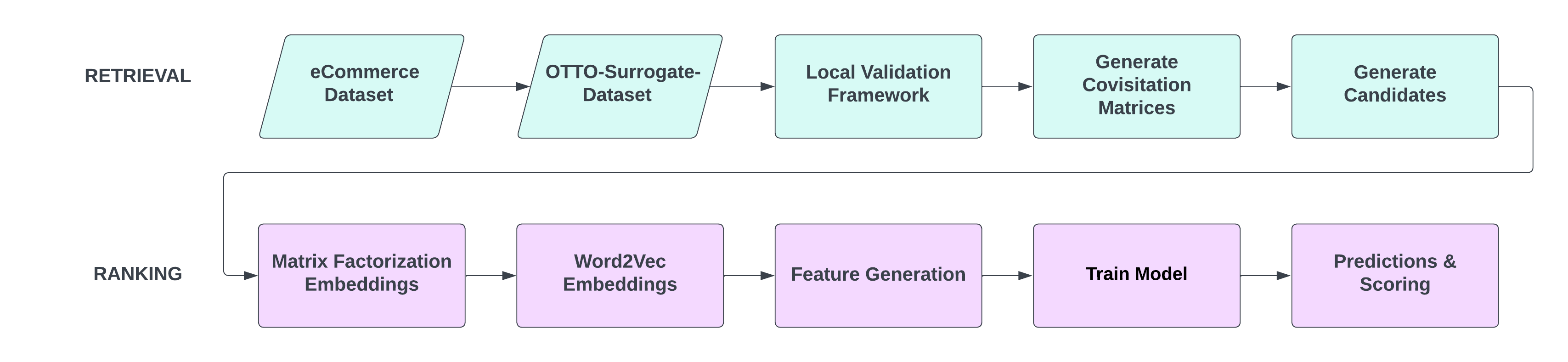
Since the OTTO Dataset was massive (train file-11 GB) and took hours for every step, I used a surrogate dataset to show the approach as a proof of concept. Most recommender systems are made up of two building blocks: Retrieval and Ranking. Retrieval generates candidates for every session in the test set, and Ranking ranks those candidates to provide the most likely aids.

The diagram illustrates the steps as part of each block.

RETRIEVAL

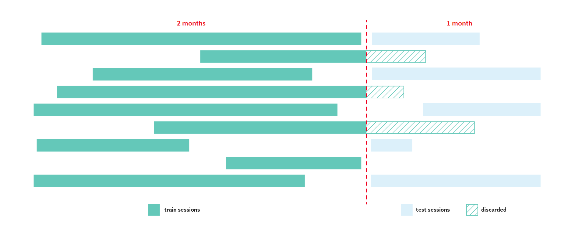
1. Creating a Local Validation Framework

Code

The surrogate ecommerce training data was approximately 4 months long - 3 months of train, and 1 month of test. From the train data, I used the last month for validation, and first 2 months for training. One thing to note is that to prevent information leakage from the future, we need to discard the validation sessions overlapping with the training sessions. Furthermore, validation data is divided into validation A and validation B (the ground truths).

2. Covisitation Matrices

Code

Covisitation matrices are based on the idea that there are products that are frequently viewed and bought together. It’s done in the following way:

• Look at pairs of events within the same session that are also within a day of each other.
• Compute the matrix by counting the global number of pairs of events. We can weight this matrix by type (clicks/orders/carts), by timestamp, or any other way.

Covisitation matrices end up looking like this:

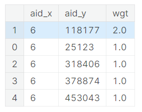
3. Generate Candidates

Code Img Source

Next, we generate candidates for each type by concatenating the tail(20) of the test session events with the most likely aids from the covisitation matrices. Most likely is determined by the weight of aid2 in the covisitation matrices.

Actually, there are a number of ways of generating candidates. In the OTTO competition, participants used covisitation matrices with handcrafted rules as above. Alternatively, we could also generate candidates using matrix factorization and a nearest neighbour search.

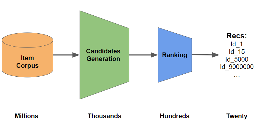
The idea behind generating candidates is to reduce the number of aids we would have to rank for each test session from millions to hundreds.

RANKING

4. Matrix Factorization and Word2Vec Embeddings

Code-MF Code-Word2Vec

Both of these steps use the train and test data to create embeddings for our aids. We can then use these embeddings to create similarity features for the ranker model.

I executed matrix factorization using Pytorch and extracted the embeddings. Then, I used a library annoy (approximate nearest neighbours, oh yeah) to get the euclidean distance between aid1 and aid2 in each of the covisitation matrices.

Word2Vec generates similar embeddings but using a different algorithm. Generally Word2Vec is used to generate linguistic similarities between words. In our case, the words are merely the aids.

5. Feature Generation

Code Img Source

This is the most important part of the entire pipeline. I would not have been able to construct features without the excellently documented code of the 34th place solution.

Here we construct 3 types of features for the candidates:

• Item features: Examples include: the count of the aid in the last week of the test session, the total and unique count of sessions that an aid appears in, the mean and std of an aid count by hour, dayofweek, or weekend, the distribution of aid by type, etc.
• User features: Examples include: session length, number of partial sessions when sessions are spread out over days, number of unique aids per session, partial sessions by type, etc.
• User-Item interaction features: These are similar to the item and user features, except that instead of grouping by just aid or session, we group by both and calculate similar metrics like unique, nunique, mean, and std.

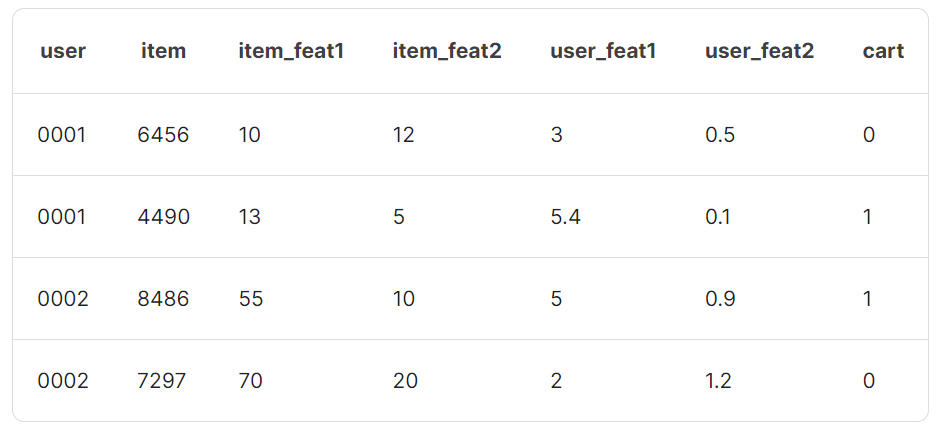
We then merge all these features with the candidate dataframes for each type, and merge the candidate dataframe with the ground truth using our validation labels, i.e., the validation B dataset. Our candidate dataframe for training should look like the following:

6. Train Model, Generate Predictions and Scoring

Code

Since the candidate file is large and divided into chunks, first we load the file into our notebook in batches and then train using XGB Ranker. We used 5 fold CV during training and create models for each type {clicks:0, carts:1, orders:2}. I used Kaggle’s 30 free GPU hours as XGBoost is quite fast on GPU.

We predictions for our local validation data for each type using our models. Scores are ranked in descending order and aids with the top 20 scores were selected as the final predictions.

Then we take our local predictions and compare to the ground truths to calculate the finall recall scores! Here is what I got for the local scores:

{
clicks recall = 0.30630826641349207
carts recall = 0.5730758544040011
orders recall = 0.7321792260692465
=============
Overall Recall = 0.6418611186040974
=============
}

If we are happy with our local validation score, we repeat this entire pipeline for the full training data. That is, we create a new candidate dataframe from Kaggle’s test data. We make item features from all 3 months of Kaggle train plus 1 month of Kaggle test. We make user features from Kaggle test. We merge the features to our candidates. Then we use our saved models to infer predictions for each type. Lastly we select 20 by sorting the predictions. Below were my test scores:

{
clicks recall = 0.3174242172714898
carts recall = 0.555169794944125
orders recall = 0.7446808510638298
=============
Overall Recall = 0.6451018708486843
=============
}

Conclusion

The biggest takeaway from the KaggleX program was that the best form of learning happens by doing. Huge shoutout again to my mentor Mensur Dlakic whose advice was vital. I hope you’ve enjoyed reading through my process. If you have any feedback, please feel free to comment on my Kaggle notebooks. Thank you!